Ultrasound-based carotid stenosis measurement and risk stratification in diabetic cohort: a deep learning paradigm

Introduction

Annually, 15 million people suffer from stroke worldwide. Amongst them, 5 million dies and the other five million are permanently disabled, thereby placing a heavy economic burden on their families and the nation (1). In the United States, the stroke figure stands at around 795,000 people annually, i.e., every 40 seconds one person suffers from stroke (2). The direct cost of medical care and treatment is approximately 33 billion United States dollars, and the indirect cost due to lost productivity is 20.6 billion United States dollars (1,2).

Stroke is caused by the obstruction of blood flow due to the narrowing (stenosis) of blood vessels of the carotid artery or cerebrovascular arteries. This narrowing is caused by the formation of plaque in the near and far walls of the carotid artery, as shown in Figure 1. This formation of plaque is due to a vessel disease called atherosclerosis (3,4). As the disease progresses with time, it causes shear stress on the arterial cap of the vessel walls causing rupture leading to thrombosis and stroke (5-7). There are many possible reasons for atherosclerosis, categorized into internal and external factors. The internal factors include genetics (8-10), age (11,12), obesity (13), hypertension (14), nutrition (15), smoking (16), diabetes mellitus (17), alcohol usage, and physical inactivity (18). The main external factor is pollution (19).

Figure 1 Anatomy of the common carotid artery and stenosis due to formation of plaque (Courtesy of Atheropoint^TM).

Non-invasive imaging techniques such as magnetic resonance imaging (MRI) or computer tomography (CT) can capture wall anatomy of the carotid artery (20). Even though MRI captures the soft tissue plaque composition (21,22), it has its own challenges such as scanning cost, gantry size, and imaging of patients that have metals in their body (such as a pacemaker). CT scan, on the other hand, involves radiation which may be dangerous for soft tissues, leading to cancer (23). In such scenarios, ultrasound (US) is an effective, low cost, non-invasive, ergonomic, radiation-free, and efficient scanning tool for the assessment of stroke and cardiovascular diseases (24-28). Among different US techniques, the two most generally used are (I) color Doppler US imaging and (II) B-mode black and white (B/W) US imaging. The color Doppler US is used to measure blood flow and pressure to detect complications in blood flow such as clots in veins and blockages in the arteries (29). However, Doppler US is dependent on velocity of blood flow which is variable. Doppler is used to measure stenosis based on pulse wave velocity (PWV) which in turn is dependent upon arterial wall stiffness (30-33). Further, Doppler spectrum gets distorted by the acoustic impedance mismatch between the fluid and the vessel walls (34) leading to low-resolution images and loss of information during color display. B-mode grayscale US, on the other hand, produces two-dimensional acoustic impedance image of the tissue (35). Currently, with the usage of harmonic and compound imaging by US original equipment manufacturers, the image resolution is very high for B-mode B/W US images. Therefore, high-resolution B-mode grayscale US scans are much preferred over color Doppler as the former can differentiate between adjacent tissues of different acoustic impedance (36).

Considerable work has been done recently which includes US scans for different applications such as lumen diameter detection and its measurement (37,38), intima-media complex (IMC) detection and its measurement (39), morphology-based tissue characterization and its risk stratification (40,41), and even linking carotid plaque burden to cardiovascular risk such as coronary syntax score (42), HbA1c (43), ABI (44,45). These techniques are an attempt to make the system automated, but these previous lumen region extraction techniques are noise sensitive (37,46,47). Also, the previously developed feature extraction algorithms were limited to a certain type of image, such as high resolution, non-curved carotids in carotid US scans, and thus cannot be generalized. As a result, the automated outputs of feature extraction techniques are not very robust. The fuzziness and low contrast of images also contribute to an erroneous output. Further, none of the previous methods are intelligence-based. The concept of training and testing paradigm using learning-based approaches seems to be missing in previous approaches. There are no strong image-based tools for stenosis measurement.

Deep learning (DL) is an emerging area which has shown to have promised in characterizing the disease (48-50). DL, unlike conventional methods, generates features internally. DL consists of multiple layers of neural networks which are trained on a large set of data where the ground truth delineations are given and then used to predict segmentations on a test set of data. Therefore, the deep layers of the DL-based system encompass an intelligence and learning-based approach towards lumen detection. Due to the combination of high-resolution B-mode US scans along with the powerful DL strategies, we hypothesize that DL-based solution will lead to more accurate stenosis severity index (SSI) measurements and risk stratifications. Thus, the objective of this study is three folds: (I) automated and accurate lumen region detection in the CCA US scans, followed by the LI-near and LI-far border detection; (II) reliable and accurate SSI measurement using NASCET criteria (51-54) and (III) risk characterization and stratification based on SSI. The novelty of this paper for lumen detection is the usage of an intelligence-based paradigm along with multiresolution framework (where images are downsampled) which further improves the speed of the DL system. In this regard, we propose a DL-based lumen detection system for characterization of stroke risk.

The DL-system implementation for SSI computation consists of four sub-stages: stage-I is the pre-processing stage where the US scans are cropped and the non-tissue region is removed in an automated fashion. Following this cropping stage, downsampling is performed for faster processing time during DL performance. Stage-II is the core of the DL-system where the features are extracted using an encoder that uses the training pool of carotid US scans. The radiologist delineated borders of the US CCA images act as the gold standard (GS) for the DL system. The binary lumen is extracted from these delineated borders and used for pixel-to-pixel classification for lumen detection. The extracted features and GS are input to the decoder, which up-samples the encoded image to match its original dimensions and classify each pixel of the original image as either lumen or non-lumen. The encoder and decoder together are part of a network architecture known as a fully convolution network (FCN) (55-57) that is used for the detection of the lumen region. Stage-III consists of LI-near and LI-far detection after up-sampling the regional carotid cropped images. Finally, stage-IV consists of risk characterization and performance evaluation.

The paper is organized as follows: section 2 presents the patient demographics and methodology, while section 3 provides the results. The statistical evaluation is presented in section 4. Section 5 presents the discussion, and finally the conclusions are presented in section 6.

Methods

Demographics

Two hundred and four patients including 157 men/47 women (77.0% vs. 23.0%) with mean age 69±11 years were selected. We analyzed 407 CCA B-mode US images from the 204 patient’s left and right carotid arteries: right carotid artery image for one patient was not available. The ethics committee of Toho University, Japan approved the IRB and informed consent was obtained from all the patients. These patients had a mean haemoglobin (HbA1c), low-density lipoprotein cholesterol, high-density lipoprotein cholesterol, total cholesterol and Cr of 5.8±1.0 mg/dL (P<0.001), 99.80±31.30 mg/dL (P=0.1735), 50.40±15.40 mg/dL (P<0.001), 174.6±37.7 mg/dL (P=0.0098) and 1.6±2.1 mg/dL (P<0.001), respectively. This cohort had 92 regular smokers. The hypertensive and high cholesterol patients were on adequate medication: statin was prescribed to 93 patients to lower the cholesterol levels, while 84 of them received renin-angiotensin system antagonists. The baseline characteristics are shown in Table 1.

Table 1 Patient demographics
Full table

US image acquisition

A sonographic scanner (Aplio XV, Aplio XG, Xario; Toshiba, Inc., Tokyo, Japan) equipped with a 7.5-MHz linear array transducer was used to examine the left and right carotid arteries. All scans were performed under the supervision of an experienced sonographer (with 15 years of experience). High-resolution images were acquired according to recommendations by the American Society of Echocardiography Carotid Intima-Media Thickness Task Force. The mean pixel resolution of the database was 0.05±0.01 mm/pixel.

Risk characterization

This dataset consisting of 204 subjects is in the subclinical atherosclerosis zone and had moderate stenosis. In this cohort, the patients did not have high stenosis (in the range of 60–80%), which is typically adopted for endarterectomy or stenting (58,59). Based on our demographics, the cohort was stratified into three risk classes: low, moderate and high-risk.

Manual lumen border delineation

The tracing of the lumen and adventitia border was implemented using ImgTracer™, user-friendly commercial software (60). A total of 15–25 edge points, covering distal, mid and proximal regions of the artery with respect to the bulb were selected in order to delineate the lumen-intima (LI)-near and LI-far boundaries of the common carotid artery (CCA). The number of points varied depending upon the length of the carotid artery. The observer had the ability to zoom in the carotid US scan for visualization of the wall region. The output of the ImgTracer™ was the ordered set of traced (x, y) coordinates.

Methodology

Our methodology originates from the spirit of an intelligence-based model for lumen border delineation. The vigor was further intensified by the role of DL-based model for feature extraction (61,62). The DL system adapted a multiresolution framework as developed before (63), however the previous work did not use DL-based techniques. Our current system is represented in Figure 2, consisting of four different stages: pre-processing stage, lumen delineation stage, LI-far, and LI-near wall delineation stage, and stenosis measurement stage. In the multiresolution stage, the images were pre-processed for removal of non-tissue region, followed by downsampling. The second stage was the core stage where DL-based model was applied to the US scans for lumen detection. The third stage consisted of the delineation of the LI-far and near walls borders. The last and the fourth stage consisted of stenosis measurement and its performance evaluation.The detailed overall system along with each of the subsystems is shown in Figure 3.

Figure 2 Global DL-system consisting of four stages: pre-processing stage, lumen detection stage, LI-near/LI-far boundary extraction system and stenosis measurement system and performance evaluation (PE). DL, deep learning.

Figure 3 Global DL-based segmentation model. DL, deep learning.

Global system

The global architecture for the DL-based system showing the four stages is presented in Figure 3. The corresponding local architecture for DL engines is shown in Figure 4. In the overall global system, the images are first pre-processed before being fed to the DL system. In this study, we have used two DL systems (55,56): DL encoder for feature extraction and DL decoder for lumen regional detection. The GS is the binary lumen extracted from radiologist delineated borders of the CCA images. Unlike previous methods which used external feature extraction techniques, the DL-based encoder generates its own features which allow it to perform better pixel-to-pixel classification. The higher-level features have better distinctive quality compared to the features obtained from the conventional feature extraction algorithms. Additionally, the depth of DL networks allows superior and better learning, which in turn leads to accurate results, compared to conventional methods. The second stage i.e., the DL-based decoder is used for lumen detection. The encoder and decoder together are part of a fully convolutional network (FCN) (57). The FCN implements an operation called skipping which allows outputs of intermediate layers to combine. This allows an effective combination of lower and higher-level features, thus allowing more effective detection. Note that the stage-II (DL stage) shown in a dotted rectangle in Figure 3 is the combination of encoder and decoder for both training-phase and testing phase of the DL system. This means for both training and testing phases, one requires encoder-decoder combination, as shown in Figure 4 (left and right half of the figures separating using the dotted line in the middle). The role of the encoder is to convolve and downsample the image with a deck of filters to generate the grayscale features, given the GS binary lumen region. On the other side, the role of the decoder is to upsample the image, while utilizing the GS in the training phase to generate the trained weights. The process of encoder-decoder combination is reused in the testing phase, where the weights from the training phase are used to encode and subsequently decode a test image without being given a ground truth segmentation. Thus, the encoder of the testing phase accepts the trained weights (left half) and incoming test image, yielding the test image feature sets. Finally, the decoder of the testing phase yields a binary lumen region by upsampling the transformed test features by using the trained weights. Note that, this is the first time that DL has been used for lumen region detection and determining LD for stenosis detection. Once the images are delineated LI-far and LI-near walls are extracted, and stenosis is estimated.

Figure 4 Local DL-based segmentation model in the training/testing paradigm. DL, deep learning.

Pre-processing stage

The pre-processing stage includes four steps: (I) automated image cropping; (II) lumen binarization; (III) image reduction/cleaning and (IV) image down-sampling. In the cropping step, all the background information, consisting of text or acquisition parameter listings, etc. is removed, ensuring the tissue region as region-of-interest (64). This process is applied to both raw US scan and corresponding ground truth (or GT) traced images. In step (II), the binarization step, binary lumen region is extracted from the GT traced images. This is based on the LI-near and LI-far borders traced by the trained physician. The third step consists of image cleaning by image reduction. Since the tissue information generally includes noisy edges on the left and right sides of the image due to the poor contact of the probe with the neck during image acquisition, one, therefore, would require cleaning these edge pixels by reducing these image regions containing these edges. This is implemented by reducing the image by 10% from left and right sides, thereby yielding crisp and sharp image. The last step consists of down-sampling to half the size for faster computation in DL framework.

Encoder phase

Encoder phase requires 13 convolution and five max-pooling layers of VGG16 network architecture (55,56) for feature extraction. One of the main advantages of using the VGG architecture is the usage of smaller kernels (convolution filters) which helps in retaining finer properties of the images in the subsequent layers. Each max-pool layer down-samples the features of its previous convolution layer. The activation function used was rectified linear unit (ReLu) which is given by:

The ReLu function provides faster training as compared to more commonly used sigmoid function, since the derivative of sigmoid is very small and therefore updates to lower level weights become negligible i.e., so-called, vanishing gradient problem. The encoder weights are initialized using pre-trained VGG weights on ImageNet. As the weights of VGG16 are trained in the training phase, high-level features are generated which are used for segmentation by the decoder. The last three layers of the VGG16 are replaced by decoder to perform the segmentation.

Decoder phase

The decoder employs three up-sampling layers of FCN. It employs skip connections which helps it to recover the full spatial resolution at the network output, paving the way for semantic segmentation. The skip operation is performed to recover spatial information lost during the down-sampling process. The skip operation is described briefly in the discussion section. Our model uses two skip operations for spatial information recovery, thereby producing highly accurate and precise segmentation output. The up-sampling/transpose convolution layers are also initialized using VGG weights. The skip connections are initialized randomly using very small weights. The encoder-decoder model is shown in Figure 5. The loss function is stated as the difference between desired and predicted probability distributions. The DL model uses this loss function to reduce the prediction error. The loss function is given by:

Figure 5 Encoder-decoder based DL architecture [reproduced with permission from (50)]. DL, deep learning.

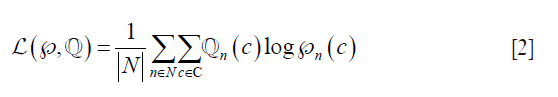
Where, is the loss function, given the prediction and ground truth , c is the current label, C is the total number of labels, n is the current image, and N is the total number of images. considers the uncertainty of the prediction based on how much it varies from the actual label is the predicted output for n^th image for class c. Similarly, is the ground truth for n^th image for class c. Note that this equation is applied for loss computation using and for each n^th image. The average loss then is computed over all the “N” number of images. A standard 50% dropout strategy is used to prevent overfitting (56).

Border extraction and carotid stenosis measurement

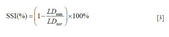
The segmented images are up-sampled to their original size. The LI-far and LI-near borders are then extracted from these segmented images. We applied NASCET criteria (46) for computing the SSI i.e., the ratio of minimum LD (LD_min) to normal LD (LD_nor) which is mathematically given as:

Results

Cross-validation protocol

The dataset consisted of 407 US scans taken from 204 patients. Three novice tracers were employed to develop three sets of GT’s. The cross-validation protocol for the DL system is shown in Figure 4. K10 cross-validation was applied, i.e., 90% of data was used for training and 10% was used for testing. Thus, the entire dataset was randomly divided into ten partitions. Ten random combinations were created from these ten partitions. Each combination consisted of two sections: the first section constituted nine parts for training i.e., 90% of the images and the other constituted one part for testing i.e., 10% of the images. The combination was fed into the DL system for training and testing phases. The process was repeated for all the other combinations. This process was repeated for all the three DL systems. At the end of the experiment, results were accumulated and the performance was computed.

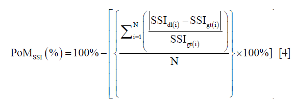
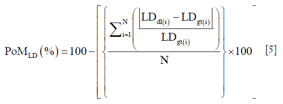
Precision-of-merit (PoM) definition for SSI and LD

The PoM and is given as:

where SSI is defined mathematically in Eq. 3 and discussed here again as ready reference i.e.,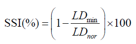

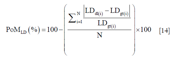
N is the total number of images in the cohort, “dl” represents the DL paradigm, “gt” represents the ground truth and “i” represents the image number. The PoM values reflect how close the automated DL method is to the manual tracings. Along the same lines, if LD_dl(i) and LD_gt(i) is the lumen diameters corresponding to DL and GTs, then the PoM based on LD which is given as:

A detailed computation of PoM_LD using polyline distance metric (PDM) is given in supplementary.

Results of LD/SSI PoMs using three DL systems

Since there are three kinds of DL methods, we have three PoMs corresponding to LD error and three PoMs corresponding to SSI. Tables 2 and 3 demonstrate the PoMs for stenosis and LDs, while the plot can be seen in Figure 6. Correspondingly, the tables and plot for DL2 are shown in Tables 4,5 and Figure 7, while for DL3, the PoMs tables and plot can be seen in Tables 6,7 and Figure 8. All the systems i.e., DL1, DL2, and DL3 were evaluated for fixed number of iterations which was empirically computed to be 4,000.

Table 2 Mean PoM stenosis (%) of DL1 w.r.t GT1
Full table

Table 3 LD absolute mean error (mm) and PoM (%) computed between DL1 and GT1
Full table

Figure 6 Percentage stenosis plot for DL1 against GT1. DL, deep learning.

Table 4 Mean PoM stenosis (%) of DL2 w.r.t GT2
Full table

Table 5 LD absolute mean error (mm) and PoM (%) computed between DL2 and GT2
Full table

Figure 7 Percentage stenosis plot for DL2 against GT2. DL, deep learning.

Table 6 Mean PoM stenosis (%) of DL3 w.r.t GT3
Full table

Table 7 LD absolute mean error (mm) and PoM (%) computed between DL3 and GT3
Full table

Figure 8 Percentage stenosis plot for DL3 against GT3. DL, deep learning.

LD/SSI estimation when trained using GT1

The experiment was conducted on 407 images based out of three sets of GTs. Almost 40% of the images showed the presence of stenosis. The results were found to be the same across all three GTs confirming that DL was able to detect stenosis accurately. It is observed from Table 2 (row #9) that the overall mean stenosis for DL1 for 407 images was 20.5%, while for GT1 it was 18.6%. It is also observed from Table 3 that the mean LD error between DL1 and GT1 was 0.19±0.27 mm (P<0.001). The stenosis plot for DL1 vs. GT1 is shown in Figure 6. It was observed that DL1 followed GT1 in the beginning for high stenosis among 20–25patients and then rises above the GT1 curve for 380 patients and finally meets GT1 at the end. The PoM between DL1 and GT1 was 96.7%.

LD/SSI estimation when trained using GT2

We perceive in Table 4 that DL2 and GT2 mean stenosis is almost same at 17.0% and 17.7%, respectively and PoM value corresponding to both DL2 and GT2 were equal to 96.1%. From Table 5, we observed that the mean LD error for DL2 and GT2 was 0.23±0.23 mm (P<0.001). The stenosis plot for DL2 vs. GT2 is shown in Figure 7. It is seen that for DL2 system, stenosis curve followed closely for all the patients when using GT2. The curve clearly showed that DL-based system gave better results when using GT2 for training.

LD/SSI estimation when trained using GT3

The mean stenosis values for DL3 and GT3 were 21.3% and 19.0%, respectively as seen in Table 6. The PoM value observed with respect to GT3 was 96.4%. The mean LD error was 0.21±0.19 mm (P<0.001) as observed from Table 7. The DL3 vs. GT3 curve is shown in Figure 8. This curve also showed that the DL3 values are in close correlation with GT3. Further, the results clearly showed having moderate stenosis.

Correlation between DL stenosis and GT stenosis for three DL systems

The regression plots for DL1 vs. GT1, DL2 vs. GT2 and DL3 vs. GT3 are shown in Figure 9A,B,C, respectively. The results show high correlation coefficients of i.e., 0.93 (P<0.0001), 0.94 (P<0.0001), and 0.93 (P<0.0001), respectively. Overall, the results clearly demonstrated that DL is better trained to predict accurate stenosis measurements with best results shown for manual reader GT2.

Figure 9 Regression plot: (A) for DL1 vs. GT1; (B) for DL2 vs. GT2; and (C) for DL3 vs. GT3. DL, deep learning.

The results clearly showed that the first two objectives of our DL-based system were successfully accomplished: the first objective being detection the lumen region followed by border delineation and second objective being stenosis computation using NASCET formulation.

Bland-Altman plots of DL-based stenosis against GT stenosis for three systems

The Bland-Altman plots for DL1 w.r.t GT1, DL2 w.r.t GT2 and DL3 w.r.t GT3 are given in Figure 10A,B,C, respectively. The plots show the means of DL and GT stenosis against the differences. The Bland-Altman plot is an effective tool to display the bias of DL and GT readings of stenosis measurement. From the three plots with respect to GT1, GT2, and G3, it is observed that the bias values were −1.8, 0.2 and −1.9, respectively showing that DL with respect to GT readings for GT1 and GT3 are consistent with each other while GT2 shows very low bias.

Figure 10 Bland-Altman plot: (A) for DL1 vs. GT1; (B) for DL2 vs. GT2; and (C) for DL3 vs. GT3. DL, deep learning.

Statistical tests, variability analysis, and risk characterization

Statistical tests are an integral part of data analysis (60,65-67). We perform the following six tests: Wilcoxon test, Mann-Whitney, paired t-test, ANOVA, Kruskal-Wallis and Friedman test. Part two consists of inter-operator variability analysis. The performance evaluation of the system is then discussed at the end of this section.

Statistical tests

Wilcoxon test, Mann-Whitney, paired t-test, ANOVA, Kruskal-Wallis and Friedman tests were performed to analyze the relationship between DL and GT readings. The P values from Wilcoxon test for DL1, DL2, and DL3 are below 0.0001. The P values from paired t-test for DL1, DL2, and DL3 were also below 0.0001. The P values from Mann-Whitney test for DL1, DL2 and DL3 were P=0.0005, P=0.0012 and P=0.0017, respectively. Therefore, for the Mann-Whitney test, the null hypothesis shows that data is taken from same distribution cannot be retained for DL1, DL2, and DL3. The analogous box plots for DL1, DL2 and DL3 systems using Wilcoxon test, Paired t-test and Mann-Whitney test are shown in Figure 11A,B,C, Figure 12A,B,C, and Figure 13A,B,C, respectively. The corresponding results are given in Tables 8-10.

Figure 11 Wilcoxon box plot: (A) for DL1 vs. GT1; (B) for DL2 vs. GT2; and (C) for DL3 vs. GT3. DL, deep learning.

Figure 12 Paired t-test box plot: (A) for DL1 vs. GT1; (B) for DL2 vs. GT2; and (C) for DL3 vs. GT3. DL, deep learning.

Figure 13 Mann-Whitney test box plot: (A) for DL1 vs. GT1; (B) for DL2 vs. GT2; and (C) for DL3 vs. GT3. DL, deep learning.

Table 8 Wilcoxon test parameters
Full table

Table 9 Paired t-test parameters
Full table

Table 10 Mann-Whitney test parameters
Full table

We performed ANOVA test (P<0.001 for DL1, P<0.001 for DL2, P<0.001 for DL3) which showed the null hypothesis is rejected such that the data was taken from same distribution cannot be retained for DL1, DL2, and DL3. Kruskal-Wallis test was also performed (P=0.466956 for DL1, P=0.448880 for DL2, P=0.449992 for DL3) which indicated that the null hypothesis is accepted such that the data is taken from same distribution can be retained for DL1, DL2, and DL3. Finally, Friedman test was performed (P<0.00001 for DL1, P<0.00001 for DL2, P<0.00001 for DL3) which indicated the null hypothesis is rejected. All results related to ANOVA, Kruskal-Wallis, Friedman tests are given in Tables 11-13.

Table 11 ANOVA test parameters
Full table

Table 12 Kruskal-Wallis test parameters
Full table

Table 13 Friedman test parameters
Full table

Inter-operator variability

The inter-operator variability shows how the trained DL systems would fare when they are plotted with each other (65,68). A regression curve was plotted between each of the trained DL. The correlation coefficient was: 0.93 (P<0.0001) for DL1 vs. DL2, 0.93 (P<0.0001) for DL1 vs. DL3 and 0.92 (P<0.0001) for DL2 vs. DL3, showing strong correlations between them. These values also prove that DL-based system in itself is stable and reproducible. The plots for each regression i.e., DL1 vs. DL2, DL1 vs. DL3 and DL2 vs. DL3 are shown in Figure 14A,B,C, respectively. The inter-operator variability between each GT is also computed. The correlation coefficient values between GT1 vs. GT2, GT1 vs. GT3, GT2 vs. GT3 are found to be 0.95, 0.96 and 0.95, respectively.

Figure 14 Regression plot: (A) for DL1 vs. DL2; (B) for DL2 vs. DL3; and (C) for DL2 vs. DL3. DL, deep learning.

Performance evaluation

The cumulative frequency distribution (CDF) plot (Figure 15) shows that for 90% of patients the stenosis error is less than 10%, while for 70% of patients it is less than 5%. From these results, it can be clearly stated that DL is robust with respect to error. The signed error CDF plots for DL1, DL2 and DL3 are shown in Figure 16A,B,C, respectively. For DL1, it shows that for 90% of patients the stenosis error is less than 8% and greater than −5%, for DL2 the stenosis error for 90% of patients’ stenosis error is less than 5% and greater than −7% and lastly, for DL3 the stenosis error is less than 9% and greater than −5% for 90% of patients. Again, our stenosis measurement system shows encouraging results.

Figure 15 CDF of stenosis error for DL1, DL2, and DL3. CDF, cumulative frequency distribution; DL, deep learning.

Figure 16 CDF of signed stenosis error: (A) for DL1; (B) for DL2; and (C) for DL3. CDF, cumulative frequency distribution; DL, deep learning.

Risk characterization and the ROC analysis for three DL systems

The third objective of our DL-based system was risk characterization depending on stenosis values. Our assumption about this cohort was in three classes which are: low, moderate and high risks. Since the maximum stenosis was 70%, we, therefore, stratified the cohort into three classes: low risk for less than 25% stenosis, moderate risk is between 25% and 50% stenosis and high risk for stenosis greater than 50%. Thus, the threshold points were 25% and 50%. A detailed comparison of threshold parameters is provided in the discussion section. Using these criteria, we computed our receiver operating characteristic (ROC) analysis for our stenosis measurement. The ROC curves for DL1, DL2, and DL3 are shown in Figure 17. The low, moderate and high-risk stenosis images are shown in Figure 18.

Figure 17 ROC plot for DL1, DL2, and DL3. ROC, receiver operating characteristic; DL, deep learning.

Figure 18 Yellow dotted lines: GT; red line: deep learning LI-near wall; green line: LI-far wall; white dotted: GT stenosis and white line: DL stenosis. Three rows: row #1 depicting low-risk stenosis for patients (A,B), row #2 depicting moderate risk stenosis for patients (C,D), and row #3 depicting high-risk stenosis for patients (E,F).

Discussion

We proposed a study on automated stenosis measurement using a DL-based paradigm on a Japanese diabetic cohort having a risk of moderate stenosis. It is due to intelligence-based learning, that the DL system outperformed the spatial-based conventional methods for accurate lumen detection and stenosis measurement from high-resolution US images. Our DL neural network system consisted of 13 deep layers that were implemented in a downsample mode to improve the performance in speed. The second stage consists of FCN that consisted of three up-sampling layers. Three observers were used for GS tracings which were then used for three DL designs, namely: DL1, DL2, and DL3. The heart of the system was the DL itself, while the pre-processing stage consisted of data preparation. The output of the DL system was automated detection of the binary lumen region which was then used for LI-near and LI-far interface edge detection to get the final lumen borders. Using the NASCET criteria, the system was then able to automatically measure the stenosis. We stratified the cohort into three classes by adapting the two threshold cut-off points for risk stratification. These two cut-offs were: 25% and 50% stenosis, dividing the cohort into three classes: low, moderate and high-risk patients. Using the GS stenosis as a response variable, our AUC’s were 0.90, 0.94 and 0.86 for DL1, DL2 and DL3, respectively. The results can be seen in Figure 18 where the test cases of high-, moderate- and low-risk stenosis from both GT and DL were presented. The comparative performance of DL-based system with contemporary techniques is provided in the next section.

Benchmarking of LD, stenosis and risk

Accurate estimation of stroke risk from examination of arterial wall is an important field of study for both neuro-radiologists, vascular US specialists such as sonologists or sonographers. By using imaging techniques there are two ways to stratify risk: the first is the study of the morphology of plaque and second, by measuring the stenosis of arterial walls (46). There have been significant studies (68) on stratification of cardiovascular risk by predicting the morphology of plaque. Lal et al. (69) used B-mode US imaging to obtain the tissue composition of plaques from carotid plaque images. el-Barghouty et al. (70) used grayscale median (GSM) to stratify between low risk and high-risk plaque from CT images. Acharya et al. (41) used ML-based approach for estimating risk from plaque composition. The stratification of plaque into asymptomatic and symptomatic has been done by using a machine learning technique on B-mode US CCA images Acharya et al. (71-73).

Another way to estimate risk is to measure the narrowing of lumen i.e., stenosis in the arterial wall (74). However, stenosis measurement requires accurate delineation of LI-far and LI-near walls from CCA artery. Many studies have been conducted to detect the lumen from US CCA images. Saba et al. (67) applied a combination of Gaussian filter and spectral analysis for lumen detection from 404 US CCA images. They used two GTs for their experiments and their corresponding LD errors were 0.25±0.24 mm and 0.27±0.26 mm (Table 14: row #1). Araki et al. (47) used both-region based and boundary-based approaches for LD detection in 300 images (Table 14: row #2 and 3). The PoM value obtained for both approaches were 97.9% and 85.2%, respectively. Araki et al. (39) again used spectral analysis for LD detection (Table 14: row #4). They used two GT’s whose mean LD errors were 0.26±0.28 and 0.27±0.26 mm. Krishna Kumar et al. (38) used a scale-space technique for 404 images using two GTs (Table 14: row #5). The LD errors were found to be 0.25±0.24 and 0.27±0.25 mm, respectively. The PoM values were 95.9% and 95.1%. Saba et al. (54) used a combination of classification tools such as level sets, region-based and boundary-based methodology for lumen detection yielding the PoM of 96.2%. Our proposed method in this study used three kinds of GTs on 407 images and obtained LD errors of 0.19±0.27 mm (P<0.001), 0.23±0.23 mm (P<0.001) and 0.21±0.19 mm (P<0.001), respectively which are best in the AtheroEdge class from AtheroPoint, Roseville, CA, USA (Table 14: row #7). The corresponding PoM values using these three GTs were 96.7%, 96.1%, and 96.4%, respectively. The PoM values are lesser than the region-based method as shown by Araki et al. (47) (Table 14: row #2) while the dataset used by the DL-based system is larger compared to the region-based method (407 US scans vs. 300 US scans). The results clearly proved that DL-based system yielded better accuracy compared to contemporary techniques.

Table 14 Benchmarking table for lumen diameter (LD)
Full table

There is however a need for standardization of risk of stroke by stenosis measurement for patients since it sets out the future course of treatment. In this regard, Randoux et al. (75) concluded that endarterectomy in patients with symptomatic moderate carotid stenosis of 50–69% produced a moderate reduction in the risk of stroke (Table 15: row #8). In another study by Nicolaides et al. (76) followed 1,115 patients with stenosis greater than 50% (using NASCET criteria) for 6–84 months. The follow-up results showed that all cardiovascular events increased for patients greater than 50% stenosis. There was a moderate rise in all cardiovascular events for patients with stenosis between 30–49% (Table 15: row #9). Kakkos et al. (77) which again showed that the inclusion stenosis criteria for carotid endarterectomy were greater than 60% (Table 15: row #10). In a similar study, Schneider et al. (78) stated that carotid endarterectomy or stenting in addition to medical therapy is still the best way to treat mostly asymptomatic patients with 60% to 99% carotid stenosis (Table 15: row #11). As discussed earlier, our dataset is primarily diabetic, in the subclinical atherosclerosis zone and has moderate stenosis. So, the dataset has been stratified into three risk zones: low-risk consisting of 25% stenosis or less, mild-risk, where stenosis ranged from 25% to 50% and high-risk when SSI was greater than 50% (Table 15: row #12).

Table 15 Benchmarking table for stenosis cut-off for stenosis risk
Full table

A short note on DL

There are two paths in the FCN: contraction path and expansion path. In the contraction path, the features are down-sampled at intermediate layers by using convolution and pooling operations. Similarly, in expansion path, the transpose of convolution is applied to up-sample the features. Skip operation is applied to skip features in the contracting path to intermediate layers in expansion path to recover spatial information lost during down-sampling in the expansion path. It is done by merging skipped features from various resolution layers in the contracting path with input features in the expansion path. As a result, highly accurate detection output is obtained from the FCN. In our model as shown in Figure 5, we have applied two skipping operations. The first set of skipped features were extracted from fourth Max Pool layer of encoder and merged with the input to second up-sampling layer in decoder. The second set of skipped features were extracted from Max Pool layer 3 of encoder and merged with the input to third up-sampling layer in decoder. DL for segmentation has also been applied for carotid intima-media thickness (49) and lumen diameter measurement (50).

Strengths and weaknesses

This is the first application of DL design in US-based stenosis measurement. The application of skip operation (where lower layer and higher layer features were combined and up-sampled) gave better detection results thereby reducing the wall errors and improving performance of the system. The inter-operator variability test was performed which showed that the proposed DL system is stable. However, there are slight differences between two curves for DL as shown in Figure 6 and Figure 8, which clearly showed that a greater number of iterations during DL training is required for better performance and reduction of overall errors. Even though we had about 400 US scans, more images are required to see its effect on the DL system.

Conclusions

This study showed the first application of DL in: (I) lumen detection; (II) near/far wall interface detection; and (III) stenosis measurement. Against conventional methods, DL showed higher accuracy with considerable error reduction. We have applied multiresolution processing before feeding data into the two-stage DL system. The performance parameters of our DL system were compared with other conventional methods implemented earlier and it showed an overall improvement in stenosis error.

Supplementary

Polyline distance metric (PDM)

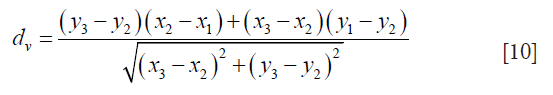
The PDM (79) is used to measure LD between LI-far and LI-near interfaces. The PDM computation is given as follows: Let the first and second borders be denoted as B₁ and B₂. Let the reference point on B₁ be vertex V₁ and the segment in B₂ be defined by vertices V₂ and V₃. Let the distance between V₁ and V₂ be d₁ and the distance between V₁ and V₃ be denoted as d₂. Let D(V₁,L) be the polyline distance between the vertex V₁:(x₁,y₁) on B₁ and line segment L formed by two points V₂:(x₂,y₂) and V₃:(x₃,y₃). Let delta (δ) be the distance of the reference point, V₁ towards the line segment L. The perpendicular distance between the line segment L and the reference point, V₁, is given by d_p. Then, the polyline distance D(V₁,L) can be defined as:

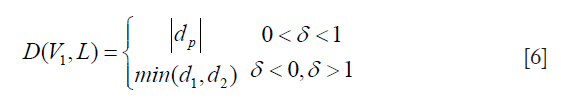
where,

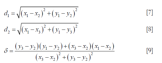
and

The process to obtain D(V₁,L) is repeated for the rest of the points of the contour C_j and is given by:

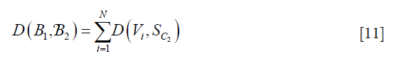
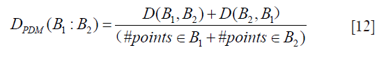
where N is the total number of points on B₁ and S_C2 is the segment on contour B₂. This algorithm is repeated in reverse, where B₂ becomes the reference boundary and B₁ becomes the segmented contour. The reverse is represented as D(B₂,B₁). Finally, by combining both D(B₁,B₂)and D(B₂,B₁), we obtain the PDM which is given by:

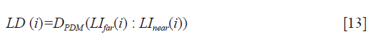
LD measurement

The LD for patient i is computed as the PDM between the LI-far wall (LI_far(i)) and LI-near (LI_near(i)) wall for the patient, which is given by:

PoM measurement

The PoM_LD(%) is computed from LD_dl and LD_gt for all patients.

Acknowledgments

None.

Footnote

Conflicts of Interest: The authors have no conflicts of interest to declare.

Ethical Statement: The authors are accountable for all aspects of the work in ensuring that questions related to the accuracy or integrity of any part of the work are appropriately investigated and resolved. The Study was approved by Toho University Japan (Ohashi Ethics Committee, Authorization No. 13-56), and all patients provided written informed consent.

References

1. Lloyd-Jones D, Adams RJ, Brown T, et al. Heart disease and stroke statistics--2010 update: a report from the American Heart Association. Circulation 2010;121:46-215.
2. Benjamin EJ, Blaha MJ, Chiuve SE, et al. Heart disease and stroke statistics-2017 update: a report from the American Heart Association. Circulation 2017;135:e146-603. [Crossref] [PubMed]
3. Suri JS, Chirinjeev K, Filippo M. Atherosclerosis disease management. 1st ed. New York: Springer Science & Business Media, 2010.
4. Saba L, Sanches JM, Pedro LM, et al. Multi-modality atherosclerosis imaging and diagnosis. 1st ed. New York: Springer, 2014.
5. Stroke report. Available online: http://www.strokeassociation.org/STROKEORG/AboutStroke/TypesofStroke/Types-of-Stroke_UCM_308531_SubHomePage.jsp
6. Spence JD. Management of asymptomatic carotid stenosis. Neurol Clin 2015;33:443-57. [Crossref] [PubMed]
7. Carr S, Farb A, William HP, et al. Atherosclerotic plaque rupture in symptomatic carotid artery stenosis. J Vasc Surg 1996;23:755-65. [Crossref] [PubMed]
8. Orho-Melander M. Genetics of coronary heart disease: towards causal mechanisms, novel drug targets and more personalized prevention. J Intern Med 2015;278:433-46. [Crossref] [PubMed]
9. Prabhakaran D, Jeemon P, Roy A. Cardiovascular diseases in India. Circulation 2016;133:1605-20. [Crossref] [PubMed]
10. Nasir K, Budoff MJ, Wong ND, et al. Family history of premature coronary heart disease and coronary artery calcification: Multi-Ethnic Study of Atherosclerosis (MESA). Circulation 2007;116:619-26. [Crossref] [PubMed]
11. Saba L, Mallarini G, Sanfilippo R, et al. Intima Media Thickness Variability (IMTV) and its association with cerebrovascular events: a novel marker of carotid atherosclerosis. Cardiovasc Diagn Ther 2012;2:10-8. [PubMed]
12. Molinari F, Zeng G, Suri JS. A state of the art review on intima–media thickness (IMT) measurement and wall segmentation techniques for carotid ultrasound. Comput Methods Programs Biomed 2010;100:201-21. [Crossref] [PubMed]
13. Ayer J, Charakida M, Deanfield JE, et al. Lifetime risk: childhood obesity and cardiovascular risk. Eur Heart J 2015;36:1371-6. [Crossref] [PubMed]
14. Hyman L, Schachat AP, He Q, et al. Hypertension, cardiovascular disease, and age-related macular degeneration. Arch Ophthalmol 2000;118:351-8. [Crossref] [PubMed]
15. D'Alessandro A, De Pergola G. Mediterranean diet and cardiovascular disease: a critical evaluation of a priori dietary indexes. Nutrients 2015;7:7863-88. [Crossref] [PubMed]
16. Critchley JA, Capewell S. Mortality risk reduction associated with smoking cessation in patients with coronary heart disease: a systematic review. JAMA 2003;290:86-97. [Crossref] [PubMed]
17. Keating ST, Plutzky J, El-Osta A. Epigenetic changes in diabetes and cardiovascular risk. Circ Res 2016;118:1706-22. [Crossref] [PubMed]
18. Haskell WL, Lee IM, Pate RR, et al. Physical activity and public health: updated recommendation for adults from the American College of Sports Medicine and the American Heart Association. Circulation 2007;116:1081-93. [Crossref] [PubMed]
19. Newby DE, Mannucci PM, Tell GS, et al. Expert position paper on air pollution and cardiovascular disease. Eur Heart J 2015;36:83-93b. [Crossref] [PubMed]
20. Suri JS, Laxminarayan S. Angiography and plaque imaging: advanced segmentation techniques. 1st ed. Boca Raton Fl: CRC Press, 2003.
21. Yuan C, Kerwin WS, Yarnykh VL, et al. MRI of atherosclerosis in clinical trials. NMR Biomed 2006;19:636-54. [Crossref] [PubMed]
22. Freilinger TM, Schindler A, Schmidt C, et al. Prevalence of nonstenosing, complicated atherosclerotic plaques in cryptogenic stroke. JACC: Cardiovasc Imaging 2012;5:397-405. [Crossref] [PubMed]
23. Saba L, Suri JS. Multi-Detector CT Imaging Handbook, Two Volume Set. 1st ed. Boca Raton, FL: CRC Press, 2013.
24. Sanches JM, Laine AF, Suri JS. Ultrasound imaging. 1st ed. New York: Springer, 2012.
25. Rangayyan RM, Suri JS. Recent Advances in Breast Imaging, Mammography, and Computer-Aided Diagnosis of Breast Cancer. 1st ed. San Francisco: SPIE Publications, 2006.
26. Andrew L, Joäao MS, Suri JS. Ultrasound Imaging: Advances and Applications. 1st ed. New York: Springer, 2012.
27. Saba L, Acharya UR, Guerriero S, et al. Ovarian Neoplasm Imaging. 1st ed. New York: Springer Science & Business Media, 2014.
28. Suri JS, Rangayyan RM, Laxminarayan S. Emerging technologies in breast imaging and mammography. 1st ed. Valencia CA: American Scientific Publishers, 2008.
29. Suri JS. Advances in diagnostic and therapeutic ultrasound imaging. 1st ed. Boston, London: Artech House, 2008.
30. Jensen JA. Estimation of blood velocities using ultrasound: a signal processing approach. 1st ed. Melbourne: Cambridge University Press, 1996.
31. Mehra S. Role of Duplex Doppler sonography in arterial stenoses. J Indian Acad Clin Med 2010;4:294-99.
32. Jones SA, Leclerc H, Chatzimavroudis GP, et al. The influence of acoustic impedance mismatch on poststenotic pulsed-doppler ultrasound measurements in a coronary artery model. Ultrasound Med Biol 1996;22:623-34. [Crossref] [PubMed]
33. Mitchell DG. Color Doppler imaging: principles, limitations, and artifacts. Radiology 1990;177:1-10. [Crossref] [PubMed]
34. Bjällmark A, Lind B, Peolsson M, et al. Ultrasonographic strain imaging is superior to conventional non-invasive measures of vascular stiffness in the detection of age-dependent differences in the mechanical properties of the common carotid artery. Eur J Echocardiogr 2010;11:630-6. [Crossref] [PubMed]
35. Benthin M, Dahl P, Ruzicka R, et al. Calculation of pulse-wave velocity using cross correlation—effects of reflexes in the arterial tree. Ultrasound Med Biol 1991;17:461-9. [Crossref] [PubMed]
36. Tole NM, Ostensen H. Basic physics of ultrasonographic imaging. 1st ed. Geneva: World Health Organization, 2005.
37. Londhe ND, Suri JS. Superharmonic Imaging for Medical Ultrasound: a Review. J Med Syst 2016;40:279-95. [Crossref] [PubMed]
38. Krishna Kumar P, Araki T, Rajan J, et al. Accurate lumen diameter measurement in curved vessels in carotid ultrasound: an iterative scale-space and spatial transformation approach. Med Biol Eng Comput 2017;55:1415-34. [Crossref] [PubMed]
39. Araki T, Kumar AM, Kumar PK, et al. Ultrasound-based automated carotid lumen diameter/stenosis measurement and its validation system. J Vasc Ultrasound 2016;40:120-34. [Crossref]
40. Molinari F, Meiburger KM, Saba L, et al. Fully Automated Dual-Snake Formulation for Carotid Intima-Media Thickness Measurement: A New Approach. J Ultrasound Med 2012;31:1123-36. [Crossref] [PubMed]
41. Acharya UR, Faust O, Sree SV, et al. An accurate and generalized approach to plaque characterization in 346 carotid ultrasound scans. IEEE Trans Instrum Meas 2012;61:1045-53. [Crossref]
42. Acharya UR, Krishnan MMR, Sree SV, et al. Plaque tissue characterization and classification in ultrasound carotid scans: a paradigm for vascular feature amalgamation. IEEE Trans Instrum Meas 2013;62:392-400. [Crossref]
43. Ikeda N, Gupta A, Dey N, et al. Improved correlation between carotid and coronary atherosclerosis SYNTAX score using automated ultrasound carotid bulb plaque IMT measurement. Ultrasound Med Biol 2015;41:1247-62. [Crossref] [PubMed]
44. Saba L, Ikeda N, Deidda M, et al. Association of automated carotid IMT measurement and HbA1c in Japanese patients with coronary artery disease. Diabetes Res Clin Pract 2013;100:348-53. [Crossref] [PubMed]
45. Ikeda N, Araki T, Sugi K, et al. Ankle–brachial index and its link to automated carotid ultrasound measurement of intima–media thickness variability in 500 Japanese coronary artery disease patients. Curr Atheroscler Rep 2014;16:393-400. [Crossref] [PubMed]
46. Nicolaides AN, Kakkos SK, Kyriacou E, et al. Asymptomatic internal carotid artery stenosis and cerebrovascular risk stratification. J Vasc Surg 2010;52:1486-96.e1. [Crossref] [PubMed]
47. Araki T, Kumar PK, Suri HS, et al. Two automated techniques for carotid lumen diameter measurement: regional versus boundary approaches. J Med Syst 2016;40:182-200. [Crossref] [PubMed]
48. Biswas M, Kuppili V, Edla DR, et al. Symtosis: A liver ultrasound tissue characterization and risk stratification in optimized deep learning paradigm Comput Methods Programs Biomed 2018;155:165-77. [Crossref] [PubMed]
49. Biswas M, Kuppili V, Araki T, et al. Deep learning strategy for accurate carotid intima-media thickness measurement: an ultrasound study on Japanese diabetic cohort. Comput Biol Med 2018;98:100-17. [Crossref] [PubMed]
50. Biswas M, Kuppili V, Saba L, et al. Deep learning fully convolution network for lumen characterization in diabetic patients using carotid ultrasound: a tool for stroke risk. Med Biol Eng Comput 2019;57:543-64. [Crossref] [PubMed]
51. Acharya UR, Faust O, Alvin AP, et al. Understanding symptomatology of atherosclerotic plaque by image-based tissue characterization. Comput Methods Programs Biomed 2013;110:66-75. [Crossref] [PubMed]
52. Fox Allan J. How to measure carotid stenosis. Radiology 1993;186:316-8. [Crossref] [PubMed]
53. Beebe HG, Salles-Cunha SX, Scissons RP, et al. Carotid arterial ultrasound scan imaging: A direct approach to stenosis measurement. J Vasc Surg 1999;29:838-44. [Crossref] [PubMed]
54. Saba L, Banchhor SK, Londhe ND, et al. Web-based accurate measurements of carotid lumen diameter and stenosis severity: An ultrasound-based clinical tool for stroke risk assessment during multicenter clinical trials. Comput Biol Med 2017;91:306-17. [Crossref] [PubMed]
55. Simonyan K, Zisserman A. Very deep convolutional networks for large-scale image recognition. arXiv preprint arXiv: 1409.1556. 2014.
56. Teichmann M, Weber M, Zoellner M, et al. Multinet: Real-time joint semantic reasoning for autonomous driving. arXiv preprint arXiv:1612.07695. 2016.
57. Long J, Shelhamer E, Darrell T. Fully convolutional networks for semantic segmentation. Proceedings of the IEEE conference on computer vision and pattern recognition. 2015:3431-40.
58. Abbott AL, Nicolaides AN. Improving outcomes in patients with carotid stenosis: call for better research opportunities and standards. Stroke 2015;46:7-8. [Crossref] [PubMed]
59. Craig DR, Meguro K, Watridge C, et al. Intracranial internal carotid artery stenosis. Stroke 1982;13:825-8. [Crossref] [PubMed]
60. Saba L, Banchhor SK, Suri HS, et al. Accurate cloud-based smart IMT measurement, its validation and stroke risk stratification in carotid ultrasound: A web-based point-of-care tool for multicenter clinical trial. Comput Biol Med 2016;75:217-34. [Crossref] [PubMed]
61. Dan C, Giusti A, Gambardella LM, et al. Deep neural networks segment neuronal membranes in electron microscopy images. Adv Neural Inf Process Syst 2012.2843-51.
62. Bar Y, Diamant I, Wolf L, et al. Chest pathology detection using deep learning with non-medical training. In 2015 IEEE 12th International Symposium on Biomedical Imaging (ISBI) 2015:294-7.
63. Molinari F, Pattichis CS, Zeng G, et al. Completely automated multiresolution edge snapper—a new technique for an accurate carotid ultrasound IMT measurement: clinical validation and benchmarking on a multi-institutional database. IEEE Trans Image Process 2012;21:1211-22. [Crossref] [PubMed]
64. Molinari F, Liboni W, Giustetto P, et al. Automatic computer-based tracings (ACT) in longitudinal 2-D ultrasound images using different scanners. J Mech Med Biol 2009;9:481-505. [Crossref]
65. Saba L, Banchhor SK, Araki T, et al. Intra-and Inter-operator Reproducibility Analysis of Automated Cloud-based Carotid Intima Media Thickness Ultrasound Measurement. J Clin Diagn Res 2018;12:11.
66. Saba L, Banchhor SK, Araki T, et al. Intra-and inter-operator reproducibility of automated cloud-based carotid lumen diameter ultrasound measurement. Indian Heart J 2018;70:649-64. [Crossref] [PubMed]
67. Saba L, Than JC, Noor NM, et al. Inter-observer variability analysis of automatic lung delineation in normal and disease patients. J Med Syst 2016;40:142-50. [Crossref] [PubMed]
68. Jensen-Urstad K, Rosfors S. A methodological study of arterial wall function using ultrasound technique. Clin Physiol 1997;17:557-67. [Crossref] [PubMed]
69. Lal BK, Hobson RW II, Pappas PJ, et al. Pixel distribution analysis of B-mode ultrasound scan images predicts histologic features of atherosclerotic carotid plaques. J Vasc Surg 2002;35:1210-7. [Crossref] [PubMed]
70. el-Barghouty N, Nicolaides A, Bahal V, et al. The identification of the high risk carotid plaque. Eur J Vasc Endovasc Surg 1996;11:470-8. [Crossref] [PubMed]
71. Araki T, Ikeda N, Shukla D, et al. A new method for IVUS-based coronary artery disease risk stratification: a link between coronary & carotid ultrasound plaque burdens. Comput Methods Programs Biomed 2016;124:161-79. [Crossref] [PubMed]
72. Acharya UR, Mookiah MR, Sree SV, et al. Atherosclerotic plaque tissue characterization in 2D ultrasound longitudinal carotid scans for automated classification: a paradigm for stroke risk assessment. Med Biol Eng Comput 2013;51:513-23. [Crossref] [PubMed]
73. Araki T, Jain PK, Suri HS, et al. Stroke risk stratification and its validation using ultrasonic Echolucent Carotid Wall plaque morphology: a machine learning paradigm. Comput Biol Med 2017;80:77-96. [Crossref] [PubMed]
74. Saba L, Jain PK, Suri HS, et al. Plaque tissue morphology-based stroke risk stratification using carotid ultrasound: a polling-based PCA learning paradigm. J Med Syst 2017;41:98-128. [Crossref] [PubMed]
75. Randoux B, Marro B, Koskas F, et al. Carotid artery stenosis: prospective comparison of CT, three-dimensional gadolinium-enhanced MR, and conventional angiography. Radiology 2001;220:179-85. [Crossref] [PubMed]
76. Nicolaides AN, Kakkos SK, Griffin M, et al. Severity of asymptomatic carotid stenosis and risk of ipsilateral hemispheric ischaemic events: results from the ACSRS study. Eur J Vasc Endovasc Surg 2005;30:275-84. [Crossref] [PubMed]
77. Kakkos SK, Sabetai M, Tegos T, et al. Risk of Stroke (ACSRS) Study Group. Silent embolic infarcts on computed tomography brain scans and risk of ipsilateral hemispheric events in patients with asymptomatic internal carotid artery stenosis. J Vasc Surg 2009;49:902-9. [Crossref] [PubMed]
78. Schneider PA, Naylor AR. Asymptomatic carotid artery stenosis—medical therapy alone versus medical therapy plus carotid endarterectomy or stenting. J Vasc Surg 2010;52:499-507. [Crossref] [PubMed]
79. Suri JS, Haralick RM, Sheehan FH. Greedy algorithm for error correction in automatically produced boundaries from low contrast ventriculograms. Pattern Anal Appl 2000;3:39-60. [Crossref]